Part 1 of 2
3. Simulations of 1850–2300 climate changeWe make simulations for 1850–2300 with radiative forcings that were used in CMIP (Climate Model Intercomparison Project) simulations reported by IPCC (2007, 2013). This allows comparison of our present simulations with prior studies. First, for the sake of later raising and discussing fundamental questions about ocean mixing and climate response time, we define climate forcings and the relation of forcings to Earth’s energy imbalance and global temperature.
3.1. Climate forcing, Earth’s energy imbalance, and climate response functionA climate forcing is an imposed perturbation of Earth’s energy balance, such as change in solar irradiance or a radiatively effective constituent of the atmosphere or surface. Non-radiative climate forcings are possible, e.g., change in Earth’s surface roughness or rotation rate, but these are small and radiative feedbacks likely dominate global climate response even in such cases. The net forcing driving climate change in our simulations (Fig. S16 in the Supplement) is almost 2 Wm(-2) at present and increases to 5–6 Wm(-2) at the end of this century, depending on how much the (negative) aerosol forcing is assumed to reduce the greenhouse gas (GHG) forcing. The GHG forcing is based on IPCC scenario A1B. “Orbital” forcings, i.e., changes in the seasonal and geographical distribution of insolation on millennial timescales caused by changes of Earth’s orbit and spin axis tilt, are near zero on global average, but they spur “slow feedbacks” of several Wm(-2), mainly change in surface reflectivity and GHGs.
When a climate forcing changes, say solar irradiance increases or atmospheric CO2 increases, Earth is temporarily out of energy balance, that is, more energy coming in than going out in these cases, so Earth’s temperature will increase until energy balance is restored. Earth’s energy imbalance is a result of the climate system’s inertia, i.e., the slowness of the surface temperature to respond to changing global climate forcing. Earth’s energy imbalance is a function of ocean mixing, as well as climate forcing and climate sensitivity, the latter being the equilibrium global temperature response to a specified climate forcing. Earth’s present energy imbalance, +0.5–1 Wm(-2) (von Schuckmann et al., 2016), provides an indication of how much additional global warming is still “in the pipeline” if climate forcings remain unchanged. However, climate change generated by today’s energy imbalance, especially the rate at which it occurs, is quite different than climate change in response to a new forcing of equal magnitude. Understanding this difference is relevant to issues raised in this paper.
The different effect of old and new climate forcings is implicit in the shape of the climate response function, R(t) where R is the fraction of the equilibrium global temperature change achieved as a function of time following imposition of a forcing. Global climate models find that a large fraction of the equilibrium response is obtained quickly, about half of the response occurring within several years, but the remainder is “recalcitrant” (Held et al., 2010), requiring many decades or even centuries for nearly complete response. Hansen (2008) showed that once a climate model’s response function R is known, based on simulations for an instant forcing, global temperature change, T(t), in response to any climate forcing history, F(t), can be accurately obtained from a simple (Green’s function) integration of R over time:

dF/dt is the annual increment of the net forcing and the integration begins before human-made climate forcing became substantial.
We use these concepts in discussing evidence that most ocean models, ours included, are too diffusive. Such excessive mixing causes the Southern and North Atlantic oceans in the models to have an unrealistically slow response to surface meltwater injection. Implications include a more imminent threat of slowdowns of Antarctic Bottom Water and North Atlantic Deep Water formation than present models suggest, with regional and global climate impacts.
3.2. Climate modelSimulations are made with an improved version of a coarse-resolution model that allows long runs at low cost: GISS (Goddard Institute for Space Studies) modelE-R. The atmosphere model is the documented modelE (Schmidt et al., 2006). The ocean is based on the Russell et al. (1995) model that conserves water and salt mass; has a free surface with divergent flow; uses a linear upstream scheme for advection; allows flow through 12 sub-resolution straits; and has background diffusivity of 0.3 cm(2) s(-1), resolution of 4° x 5° and 13 layers that increase in thickness with depth.
However, the ocean model includes simple but significant changes, compared with the version documented in simulations by Miller et al. (2014). First, an error in the calculation of neutral surfaces in the Gent–McWilliams (GM; Gent and McWilliams, 1990) mesoscale eddy parameterization was corrected; the resulting increased slope of neutral surfaces provides proper leverage to the restratification process and correctly orients eddy stirring along those surfaces.
Second, the calculation of eddy diffusivity K(meso) for GM following Visbeck et al. (1997) was simplified to use a length scale independent of the density structure (J. Marshall, personal communication, 2012):
Kmeso = C/[TEady x f (latitude)], (2)
where C =(27.9 km)(2), Eady growth rate 1=TEady = {│S x N│}, S is the neutral surface slope, N the Brunt–Väisälä frequency, {} signifies averaging over the upper D meters of ocean depth, D = min(max(depth,400 m), 1000 m), and f (latitude)=max(0.1, sin(│latitude│)) (1) to qualitatively mimic the larger values of the Rossby radius of deformation at low latitudes. These choices for Kmeso, whose simplicity is congruent with the use of a depth-independent eddy diffusivity and the use of 1=T(eady) as a metric of eddy energy, result in the zonal average diffusivity shown in Fig. 1. Third, the so-called nonlocal terms in the KPP mixing parameterization (Large et al., 1994) were activated. All of these modifications tend to increase the ocean stratification, and in particular the Southern Ocean state is fundamentally improved. For example, we show in Sect. 3.8.5 that our current model produces Antarctic Bottom Water on the Antarctic coastline, as observed, rather than in the middle of the Southern Ocean as occurs in many models, including the GISS-ER model documented in CMIP5. However, although overall realism of the ocean circulation is much improved, significant model deficiencies remain, as we will describe.
The simulated Atlantic meridional overturning circulation (AMOC) has maximum flux that varies within the range ~14–18 Sv in the model control run (Figs. 2 and 3). AMOC strength in recent observations is 17.5 ±1.6 Sv (Baringer et al., 2013; Srokosz et al., 2012), based on 8 years (2004– 2011) of data for an in situ mooring array (Rayner et al., 2011; Johns et al., 2011).
Ocean model control run initial conditions are climatology for temperature and salinity (Levitus and Boyer, 1994; Levitus et al., 1994); atmospheric composition is that of 1880 (Hansen et al., 2011). Overall model drift from control run initial conditions is moderate (see Fig. S1 for planetary energy imbalance and global temperature), but there is drift in the North Atlantic circulation. The AMOC circulation cell initially is confined to the upper 3 km at all latitudes (1st century in Figs. 2 and 3), but by the 5th century the cell reaches deeper at high latitudes.
Zonal–mean mesoscale diffusivity (m2/s)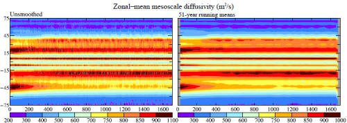 Figure 1. Zonal-mean mesoscale diffusivity (m(2) s(-1)) versus time in control run.Atlantic meridional overturning circulation (Sv)
 Figure 2. AMOC (Sv) in the 1st, 5th, 10th, 15th and 20th centuries of the control run.
Atmospheric and surface climate in the present model is similar to the documented modelE-R, but because of changes to the ocean model we provide several diagnostics in the Supplement. A notable flaw in the simulated surface climate is the unrealistic double precipitation maximum in the tropical Pacific (Fig. S2). This double Intertropical Convergence Zone (ITCZ) occurs in many models and may be related to cloud and radiation biases over the Southern Ocean (Hwang and Frierson, 2013) or deficient low level clouds in the tropical Pacific (de Szoeke and Xie, 2008). Another flaw is unrealistic hemispheric sea ice, with too much sea ice in the Northern Hemisphere and too little in the Southern Hemisphere (Figs. S3 and S4). Excessive Northern Hemisphere sea ice might be caused by deficient poleward heat transport in the Atlantic Ocean (Fig. S5). However, the AMOC has realistic strength and Atlantic meridional heat transport is only slightly below observations at high latitudes (Fig. S5). Thus we suspect that the problem may lie in sea ice parameterizations or deficient dynamical transport of ice out of the Arctic. The deficient Southern Hemisphere sea ice, at least in part, is likely related to excessive poleward (southward) transport of heat by the simulated global ocean (Fig. S5), which is related to deficient northward transport of heat in the modeled Atlantic Ocean (Fig. S5).
A key characteristic of the model and the real world is the response time: how fast does the surface temperature adjust to a climate forcing? ModelE-R response is about 40% in 5 years (Fig. 4) and 60% in 100 years, with the remainder requiring many centuries. Hansen et al. (2011) concluded that most ocean models, including modelE-R, mix a surface temperature perturbation downward too efficiently and thus have a slower surface response than the real world. The basis for this conclusion was empirical analysis using climate response functions, with 50, 75 and 90% response at year 100 for climate simulations (Hansen et al., 2011). Earth’s measured energy imbalance in recent years and global temperature change in the past century revealed that the response function with 75% response in 100 years provided a much better fit with observations than the other choices. Durack et al. (2012) compared observations of how rapidly surface salinity changes are mixed into the deeper ocean with the large number of global models in CMIP3, reaching a similar conclusion, that the models mix too rapidly.
Our present ocean model has a faster response on 10–75- year timescales than the old model (Fig. 4), but the change is small. Although the response time in our model is similar to that in many other ocean models (Hansen et al., 2011), we believe that it is likely slower than the real-world response on timescales of a few decades and longer. A too slow surface response could result from excessive small-scale mixing. We will argue, after the studies below, that excessive mixing likely has other consequences, e.g., causing the effect of freshwater stratification on slowing Antarctic Bottom Water (AABW) formation and growth of Antarctic sea ice cover to occur 1–2 decades later than in the real world. Similarly, excessive mixing probably makes the AMOC in the model less sensitive to freshwater forcing than the real-world AMOC.
3.3. Experiment definition: exponentially increasing freshwaterAtlantic meridional overturning circulation (Sv): Control run (2000 years)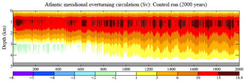 Figure 3. Annual mean AMOC (Sv) at 28 N in the model control run.Climate response functions
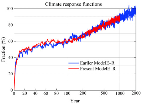 Figure 4. Climate response function, R.t/, i.e., the fraction (%) of equilibrium surface temperature response for GISS modelE-R based on a 2000-year control run (Hansen et al., 2007a). Forcing was instant CO2 doubling with fixed ice sheets, vegetation distribution, and other long-lived GHGs.
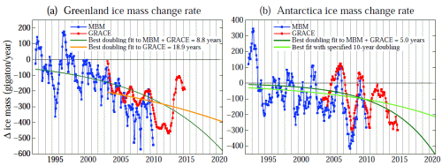
Freshwater injection is 360 Gt year(-1) (1 mm sea level) in 2003–2015, then grows with 5-, 10- or 20-year doubling time (Fig. 5) and terminates when global sea level reaches 1 or 5 m. Doubling times of 10, 20 and 40 years, reaching meter-scale sea level rise in 50, 100, and 200 years may be a more realistic range of timescales, but 40 years yields little effect this century, the time of most interest, so we learn more with less computing time using the 5-, 10- and 20-year doubling times. Observed ice sheet mass loss doubling rates, although records are short, are ~ 10 years (Sect. 5.1). Our sharp cutoff of melt aids separation of immediate forcing effects and feedbacks.
We argue that such a rapid increase in meltwater is plausible if GHGs keep growing rapidly. Greenland and Antarctica have outlet glaciers in canyons with bedrock below sea level well back into the ice sheet (Fretwell et al., 2013; Morlighem et al., 2014; Pollard et al., 2015). Feedbacks, including ice sheet darkening due to surface melt (Hansen et al., 2007b; Robinson et al., 2012; Tedesco et al., 2013; Box et al., 2012) and lowering and thus warming of the near-coastal ice sheet surface, make increasing ice melt likely. Paleoclimate data reveal sea level rise of several meters in a century (Fairbanks, 1989; Deschamps et al., 2012). Those cases involved ice sheets at lower latitudes, but 21st century climate forcing is larger and increasing much more rapidly.
Radiative forcings (Fig. S16a, b) are from Hansen et al. (2007c) through 2003 and IPCC scenario A1B for later GHGs. A1B is an intermediate IPCC scenario over the century, but on the high side early this century (Fig. 2 of Hansen et al., 2007c).We add freshwater to the North Atlantic (ocean area within 52–72° N and 15° E–65° N) or Southern Ocean (ocean south of 60° S), or equally divided between the two oceans. Ice sheet discharge (icebergs plus meltwater) is mixed as freshwater with mean temperature -15° C into the top three ocean layers (Fig. S6).
3.4. Simulated surface temperature and energy balanceWe present surface temperature and planetary energy balance first, thus providing a global overview. Then we examine changes in ocean circulation and compare results with prior studies.
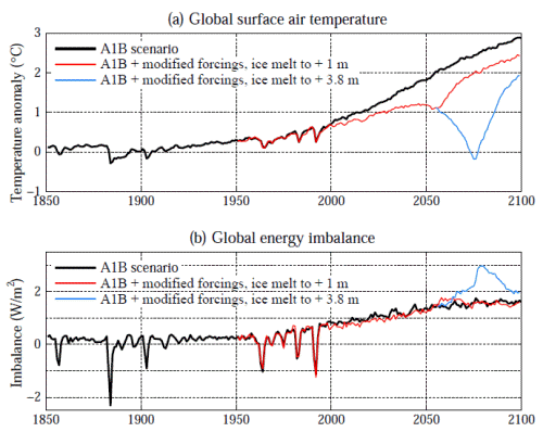
Temperature change in 2065, 2080 and 2096 for 10-year doubling time (Fig. 6) should be thought of as results when sea level rise reaches 0.6, 1.7 and 5 m, because the dates depend on initial freshwater flux. Actual current freshwater flux may be about a factor of 4 higher than assumed in these initial runs, as we will discuss, and thus effects may occur ~20 years earlier. A sea level rise of 5m in a century is about the most extreme in the paleo-record (Fairbanks, 1989; Deschamps et al., 2012), but the assumed 21st century climate forcing is also more rapidly growing than any known natural forcing.
Meltwater injected into the North Atlantic has larger initial impact, but Southern Hemisphere ice melt has a greater global effect for larger melt as the effectiveness of more meltwater in the North Atlantic begins to decline. The global effect is large long before sea level rise of 5 m is reached. Meltwater reduces global warming about half by the time sea level rise reaches 1.7 m. Cooling due to ice melt more than eliminates A1B warming in large areas of the globe.
(a) Freshwater melt flux / (b) Resulting sea level rise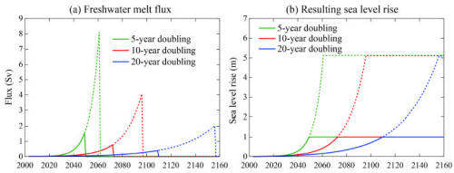 Figure 5. (a) Total freshwater flux added in the North Atlantic and Southern oceans and (b) resulting sea level rise. Solid lines for 1 m sea level rise, dotted for 5 m. One sverdrup (Sv) is 10(6) m(3) s(-1), which is ~3 x 10(4) Gt year(-1).Annual mean surface air temperature change ( C)
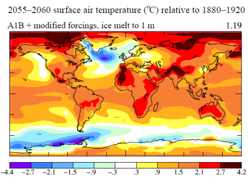
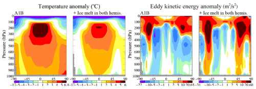
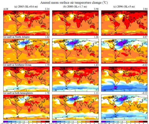 Figure 6. Surface air temperature (°C) relative to 1880–1920 in (a) 2065, (b) 2080, and (c) 2096. Top row is IPCC scenario A1B. Ice melt with 10-year doubling is added in other scenarios.
The large cooling effect of ice melt does not decrease much as the ice melting rate varies between doubling times of 5, 10 or 20 years (Fig. 7a). In other words, the cumulative ice sheet melt, rather than the rate of ice melt, largely determines the climate impact for the range of melt rates covered by 5-, 10- and 20-year doubling times. Thus if ice sheet loss occurs even to an extent of 1.7m sea level rise (Fig. 7b), a large impact on climate and climate change is predicted.
Greater global cooling occurs for freshwater injected into the Southern Ocean, but the cooling lasts much longer for North Atlantic injection (Fig. 7a). That persistent cooling, mainly at Northern Hemisphere middle and high latitudes (Fig. S7), is a consequence of the sensitivity, hysteresis effects, and long recovery time of the AMOC (Stocker and Wright, 1991; Rahmstorf, 1995, and earlier studies referenced therein). AMOC changes are described below.
(a) Global surface air temperature / (b) Global energy imbalance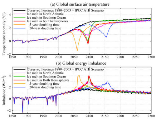 Figure 7. (a) Surface air temperature (°C) relative to 1880–1920 for several scenarios. (b) Global energy imbalance (Wm(-2)/ for the same scenarios.
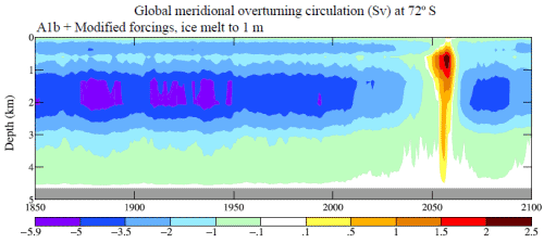
When freshwater injection in the Southern Ocean is halted, global temperature jumps back within two decades to the value it would have had without any freshwater addition (Fig. 7a). Quick recovery is consistent with the Southern Ocean-centric picture of the global overturning circulation (Fig. 4; Talley, 2013), as the Southern Ocean meridional overturning circulation (SMOC), driven by AABW formation, responds to change in the vertical stability of the ocean column near Antarctica (Sect. 3.7) and the ocean mixed layer and sea ice have limited thermal inertia.
Cooling from ice melt is largely regional, temporary, and does not alleviate concerns about global warming. Southern Hemisphere cooling is mainly in uninhabited regions. Northern Hemisphere cooling increases temperature gradients that will drive stronger storms (Sect. 3.9).
Global cooling due to ice melt causes a large increase in Earth’s energy imbalance (Fig. 7b), adding about +2Wm(-2), which is larger than the imbalance caused by increasing GHGs. Thus, although the cold freshwater from ice sheet disintegration provides a negative feedback on regional and global surface temperature, it increases the planet’s energy imbalance, thus providing more energy for ice melt (Hansen, 2005). This added energy is pumped into the ocean.
Increased downward energy flux at the top of the atmosphere is not located in the regions cooled by ice melt. However, those regions suffer a large reduction of net incoming energy (Fig. 8a). The regional energy reduction is a consequence of increased cloud cover (Fig. 8b) in response to the colder ocean surface. However, the colder ocean surface reduces upward radiative, sensible and latent heat fluxes, thus causing a large (~50 Wm(-2)) increase in energy into the North Atlantic and a substantial but smaller flux into the Southern Ocean (Fig. 8c).
Below we conclude that the principal mechanism by which this ocean heat increases ice melt is via its effect on ice shelves. Discussion requires examination of how the freshwater injections alter the ocean circulation and internal ocean temperature.
3.5. Simulated Atlantic meridional overturning circulation (AMOC)Broecker’s articulation of likely effects of freshwater outbursts in the North Atlantic on ocean circulation and global climate (Broecker, 1990; Broecker et al., 1990) spurred quantitative studies with idealized ocean models (Stocker and Wright, 1991) and global atmosphere–ocean models (Manabe and Stouffer, 1995; Rahmstorf 1995, 1996). Scores of modeling studies have since been carried out, many reviewed by Barreiro et al. (2008), and observing systems are being developed to monitor modern changes in the AMOC (Carton and Hakkinen, 2011).
Change in 2080 relative to 1880–1920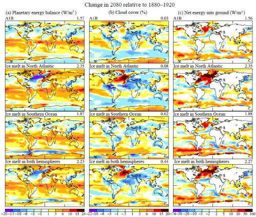 Figure 8. Change in 2080 (mean of 2078–2082), relative to 1880–1920, of annual mean (a) planetary energy balance (Wm(-2)), (b) cloud cover (%), and (c) net energy into ground (Wm(-2)) for the same scenarios as Fig. 6.
Our climate simulations in this section are five-member ensembles of runs initiated at 25-year intervals at years 901– 1001 of the control run. We chose this part of the control run because the planet is then in energy balance (Fig. S1), although by that time model drift had altered the slow deep-ocean circulation. Some model drift away from initial climatological conditions is inevitable, as all models are imperfect, and we carry out the experiments with cognizance of model limitations. However, there is strong incentive to seek basic improvements in representation of physical processes to reduce drift in future versions of the model.
GHGs alone (scenario A1B) slow AMOC by the early 21st century (Fig. 9), but variability among individual runs (Fig. S8) would make definitive detection difficult at present. Freshwater injected into the North Atlantic or in both hemispheres shuts down the AMOC (Fig. 9, right side). GHG amounts are fixed after 2100 and ice melt is zero, but after two centuries of stable climate forcing the AMOC has not recovered to its earlier state. This slow recovery was found in the earliest simulations by Manabe and Stouffer (1994) and Rahmstorf (1995, 1996).
Freshwater injection already has a large impact when ice melt is a fraction of 1m of sea level. By the time sea level rise reaches 59 cm (2065 in the present scenarios), when freshwater flux is 0.48 Sv, the impact on AMOC is already large, consistent with the substantial surface cooling in the North Atlantic (Fig. 6).
3.6. Comparison with prior simulationsAMOC sensitivity to GHG forcing has been examined extensively based on CMIP studies. Schmittner et al. (2005) found that AMOC weakened 25±25% by the end of the 21st century in 28 simulations of 9 different models forced by the A1B emission scenario. Gregory et al. (2005) found 10– 50% AMOC weakening in 11 models for CO2 quadrupling (1% year(-1) increase for 140 years), with largest decreases in models with strong AMOCs. Weaver et al. (2007) found a 15–31% AMOC weakening for CO2 quadrupling in a single model for 17 climate states differing in initial GHG amount. AMOC in our model weakens 30% in the century between 1990–2000 and 2090–2100, the period used by Schmittner et al. (2005), for A1B forcing (Fig. S8). Thus our model is more sensitive than the average but within the range of other models, a conclusion that continues to be valid in comparison with 10 CMIP5 models (Cheng et al., 2013).
Atlantic meridional overturning circulation (Sv) at 28° N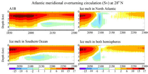 Figure 9. Ensemble-mean AMOC (Sv) at 28° N versus time for the same four scenarios as in Fig. 6, with ice melt reaching 5m at the end of the 21st century in the three experiments with ice melt.
AMOC sensitivity to freshwater forcing has not been compared as systematically among models. Several studies find little impact of Greenland melt on AMOC (Huybrechts et al., 2002; Jungclaus et al., 2006; Vizcaino et al., 2008) while others find substantial North Atlantic cooling (Fichefet et al., 2003; Swingedouw et al., 2007; Hu et al., 2009, 2011). Studies with little impact calculated or assumed small ice sheet melt rates, e.g., Greenland contributed only 4 cm of sea level rise in the 21st century in the ice sheet model of Huybrechts et al. (2002). Fichefet et al. (2003), using nearly the same atmosphere–ocean model as Huybrechts et al. (2002) but a more responsive ice sheet model, found AMOC weakening from 20 to 13 Sv late in the 21st century, but separate contributions of ice melt and GHGs to AMOC slowdown were not defined.
Hu et al. (2009, 2011) use the A1B scenario and freshwater from Greenland starting at 1mm sea level per year increasing 7% year(-1), similar to our 10-year doubling case. Hu et al. keep the melt rate constant after it reaches 0.3 Sv (in 2050), yielding 1.65m sea level rise in 2100 and 4.2m in 2200. Global warming found by Hu et al. for scenario A1B resembles our result but is 20–30% smaller (compare Fig. 2b of Hu et al., 2009 to our Fig. 6), and cooling they obtain from the freshwater flux is moderately less than that in our model. AMOC is slowed about one-third by the latter 21st century in the Hu et al. (2011) 7% year(-1) experiment, comparable to our result.
General consistency holds for other quantities, such as changes of precipitation. Our model yields southward shifting of the Intertropical Convergence Zone (ITCZ) and intensification of the subtropical dry region with increasing GHGs (Fig. S9), as has been reported in modeling studies of Swingedouw et al. (2007, 2009). These effects are intensified by ice melt and cooling in the North Atlantic region (Fig. S9).
A recent five-model study (Swingedouw et al., 2014) finds a small effect on AMOC for 0.1 Sv Greenland freshwater flux added in 2050 to simulations with a strong GHG forcing. Our larger response is likely due, at least in part, to our freshwater flux reaching several tenths of a sverdrup.
3.7. Pure freshwater experimentsWe assumed, in discussing the relevance of these experiments to Eemian climate, that effects of freshwater injection dominate over changing GHG amount, as seems likely because of the large freshwater effect on sea surface temperatures (SSTs) and sea level pressure. However, Eemian CO2 was actually almost constant at ~275 ppm (Luthi et al., 2008). Thus, to isolate effects better, we now carry out simulations with fixed GHG amount, which helps clarify important feedback processes.
Our pure freshwater experiments are five-member ensembles starting at years 1001, 1101, 1201, 1301, and 1401 of the control run. Each experiment ran 300 years. Freshwater flux in the initial decade averaged 180 km(3) year(-1) (0.5mm sea level) in the hemisphere with ice melt and increased with a 10-year doubling time. Freshwater input is terminated when it reaches 0.5m sea level rise per hemisphere for three five-member ensembles: two ensembles with injection in the individual hemispheres and one ensemble with input in both hemispheres (1m total sea level rise). Three additional ensembles were obtained by continuing freshwater injection until hemispheric sea level contributions reached 2.5 m. Here we provide a few model diagnostics central to discussions that follow. Additional results are provided in Figs. S10–S12.
The AMOC shuts down for Northern Hemisphere freshwater input yielding 2.5m sea level rise (Fig. 10). By year 300, more than 200 years after cessation of all freshwater input, AMOC is still far from full recovery for this large freshwater input. On the other hand, freshwater input of 0.5 m does not cause full shutdown, and AMOC recovery occurs in less than a century.
Atlantic meridional overturning circulation (Sv) at 28° N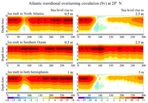 Figure 10. Ensemble-mean AMOC (Sv) at 28° N versus time for six pure freshwater forcing experiments.
Global temperature change (Fig. 11) reflects the fundamentally different impact of freshwater forcings of 0.5 and 2.5 m. The response also differs greatly depending on the hemisphere of the freshwater input. The case with freshwater forcing in both hemispheres is shown only in the Supplement because, to a good approximation, the response is simply the sum of the responses to the individual hemispheric forcings (see Figs. S10–S12). The sum of responses to hemispheric forcings moderately exceeds the response to global forcing.
Global cooling continues for centuries for the case with freshwater forcing sufficient to shut down the AMOC (Fig. 11). If the forcing is only 0.5m of sea level, the temperature recovers in a few decades. However, the freshwater forcing required to reach the tipping point of AMOC shutdown may be less in the real world than in our model, as discussed below. Global cooling due to freshwater input on the Southern Ocean disappears in a few years after freshwater input ceases (Fig. 11), for both the smaller (0.5m of sea level) and larger (2.5 m) freshwater forcings.
Injection of a large amount of surface freshwater in either hemisphere has a notable impact on heat uptake by the ocean and the internal ocean heat distribution (Fig. 12). Despite continuous injection of a large amount of very cold (-15° C) water in these pure freshwater experiments, substantial portions of the ocean interior become warmer. Tropical and Southern Hemisphere warming is the well-known effect of reduced heat transport to northern latitudes in response to the AMOC shutdown (Rahmstorf, 1996; Barreiro et al., 2008).
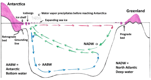
However, deep warming in the Southern Ocean may have greater consequences. Warming is maximum at grounding line depths (~1–2 km) of Antarctic ice shelves (Rignot and Jacobs, 2002). Ice shelves near their grounding lines (Fig. 13 of Jenkins and Doake, 1991) are sensitive to temperature of the proximate ocean, with ice shelf melting increasing 1m per year for each 0.1° C temperature increase (Rignot and Jacobs, 2002). The foot of an ice shelf provides most of the restraining force that ice shelves exert on landward ice (Fig. 14 of Jenkins and Doake, 1991), making ice near the grounding line the buttress of the buttress. Pritchard et al. (2012) deduce from satellite altimetry that ice shelf melt has primary control of Antarctic ice sheet mass loss.
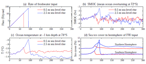
Thus we examine our simulations in more detail (Fig. 13). The pure freshwater experiments add 5mm sea level in the first decade (requiring an initial 0.346 mm year (-1) for 10-year doubling), 10 mm in the second decade, and so on (Fig. 13a). Cumulative freshwater injection reaches 0.5m in year 68 and 2.5 m in year 90.
Global surface air temperature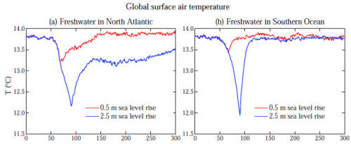 Figure 11. Ensemble-mean global surface air temperature (°C) for experiments (years on x axis) with freshwater forcing in either the North Atlantic Ocean (left) or the Southern Ocean (right).Ocean temperature change ( C) in pure freshwater experiment
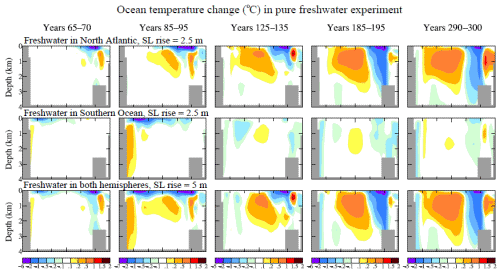 Figure 12. Change of ocean temperature (°C) relative to control run due to freshwater input that reaches 2.5 m of global sea level in a hemisphere (thus 5 m sea level rise in the bottom row).
Antarctic Bottom Water (AABW) formation is reduced ~20 % by year 68 and ~50 % by year 90 (Fig. 13b). When freshwater injection ceases, AABW formation rapidly regains full strength, in contrast to the long delay in reestablishing North Atlantic Deep Water (NADW) formation after AMOC shutdown. The Southern Ocean mixed-layer response time dictates the recovery time for AABW formation. Thus rapid recovery also applies to ocean temperature at depths of ice shelf grounding lines (Fig. 13c). The rapid response of the Southern Ocean meridional overturning circulation (SMOC) implies that the rate of freshwater addition to the mixed layer is the driving factor.
Freshwater flux has little effect on simulated Northern Hemisphere sea ice until the 7th decade of freshwater growth (Fig. 13d), but Southern Hemisphere sea ice is more sensitive, with substantial response in the 5th decade and large response in the 6th decade. Below we show that “5th decade” freshwater flux (2880 Gt year(-1)) is already relevant to the Southern Ocean today.